| This document is available in: English Castellano Deutsch Francais Italiano |
![[Photo of the Author]](../../common/images/Antonio-C.gif)
by Antonio Castro <acastro(at)ctv.es> About the author: Computer Science is my profession and also part of my free time. I like to share my hobby, as everyone probably does. I admit it! I am one of those strange characters who dislikes windoze, at least MSDOS has the category of a toy that is least pretentious of its capabilities and does not fill your computer of numerous files that where you never now if they are useful and what they are good for. Translated to English by: Miguel A Sepulveda <sepulveda(at)linuxfocus.org> Content: |
![[Illustration]](../../common/images/illustration11.gif)
Abstract:
This time we explore how to design recursive structures with Povray and how to create beautiful images with this technique.
CGS primitives are elementary solid objects that can be combined into more complex models. The final combination can be grouped and transformed using scaling, translations, rotations transformations or filling in textures, etc... It is not necessary to to apply each of these transformations to each and everyone of the elementary primitives in the combined model.
There are four methods to combine CGS primitives, and there is a fifth complement method that applies to single primitives:
As in the union, except that the internal surfaces of A and B are removed. If the objects are not translucid this features is of no use.
In the following examples we will use several of these operations to build solid models. I recommend to build models by adding first all the elements needed to make the overall volume and then using intersection operations to eliminate the undesired parts.
#define EatenApple = intersection {
      object { WholeApple }
      object { Bite1 inverse }
      object { Bite2 inverse }
}
|
When primitives objects in a solid model have common surfaces there may be problems of rendering points in one of the other surface due to machine precission. This problem can be worked around by introducing a very small translation in one the objects to clearly distinguish to which object the surface belongs to.
The elements in a scene are described generally in an arbitrary order. Nevertheless there are occasions when it is very convenient to implement procedural loops to create iterative structures, for example. Loops can be implemented in Povray using several methods. One method is the loop flow control directive provided by the language itself.
The loop flow control is just one of many directives of the POVRAY programming interface. Some while ago we mentioned other directives like #declare and #include and we characterized many others as of minor importance. The example that follows was edited directly in POVRAY and I must confess this is the first time I use the loop flow control directive. The reason is that often it is possible to achieve the same result by generating the POVRAY source with a separate program (C or C++) that has loop flow control statements (for loop). We will see at some point an example of this technique.
The reader with C experience will understand that Povray's programming interface is not as elegant as other general purpose programming languages (C, C++). This should not come as a surprise because POVRAY was designed as a language for the description of scenes, and the flow control directives were later additions. Similarly, POVRAY includes directives for performing complex mathematical operations and all kind of loops. Personally I believe it is fantastic that POVRAY includes all these operations, on the other hand they are not really not absolutely necessary since we can alway execute them externally in more powerful programming languages. I do not see how performing these operations externally or internally makes any difference to the final artistic value of the composition. For me the most important issue is the quality of the final image. To a lesser extent it should also be a factor the time and effort required to develop and process the image. Users more familiar with general purpose languages may feel better generating POVRAY files through them, others without programming experience perhaps would feel more comfortable writing directly in POVRAY. Also for simple images direct editing in POVRAY is easier while for complex scenes the generation of POVRAY files by other programs may be better. We will explore both methods and let the reader pick accordingly.
Many scenes can be designed starting from a simple idea. After a first implementation we may decide to change some value or use approximations to achieve a better result. So trial and error is an integral part of scene design in POVRAY. At the beginning of this series of articles we offered readers a simple script-tool (POV) to facilitate the generation of images, but the reader should not think that this little script is sufficient. Often times you will need plain paper, pencil and a calculator. In many occasions there is no choice because our designs involved 3D geometries, some knowledge of special geometry and trigonometry are fundamental in order to achieve certain effects. Generally it is sufficient to know a few formulas, so let us remember some basic trigonometric relationships:
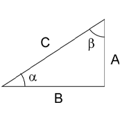 sin(a) = A / C = (Opposite side
/ Hypotenuse)
 Therefore:
A = sin(a)/CNext as a reminder we will tabulate the main domains for the trigonometric functions as a function of the quadrant:
| Quadrant | Sine | Cosine | Tangent |
| 0 .. 90 | 0 .. +1 | +1 .. 0 | 0 .. +Infinity |
| 90 .. 180 | +1 .. 0 | 0 .. -1 | -Infinity .. 0 |
| 180 .. 270 | 0 .. -1 | -1 .. 0 | 0 .. +Infinity |
| 270 .. 360 | -1 .. 0 | 0 .. +1 | -Infinity .. 0 |
This last relationship is not uniquely defined. The angle alpha is undetermined by +/- 180 degrees.Computationally it is preferably to use this:
a = atan2(A,B)Finally the distance from P1(x1,y1,z1) to P2(x2,y2,z2) is
D = sqrt( (x2-x1)^2 + (y2-y1)^2 + (z2-z1)^2 )
There are many usefull trigonometric relationships but the ones already reviewed should be sufficient for most cases. The implicit trigonometric functions implemented in POVRAY assume by default angles in radians. The conversion function radians(alpha) transforms degrees to radians. Unfortunately POVRAY is not consistent, for example rotations are measured in degrees! :-(
In the following example we use some very basic trigonometry. The spikes in the sea-urchin are placed very conveniently, and this effect cannot be easily achieved by chance. The designer has to think about an algorithm to place the spikes exactly and implement it with a clear idea of the final 3D configuration. The source code for the example is sufficiently documented, so it is not worth to make further comments here. This example is a clear case where a loop algorithm applies. Whether the designer decides to implement the loop within POVRAY or outside via a C-program is a matter of personal choice.
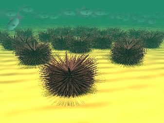
Here are the sources for the fish. They are modeled using CGS primitives as previously described.
Next comes the sources for the remaining scene. The most peculiar issue here is the definition of the sea-urchin (erizo in Spanish) that without a doubt are the principal characters in the composition:
A number of effects in this example are completely new, for example the surface effects on the sand (waves on the sand), the atmospheric effects (a fog of green marine color very thick and very humid) and the complex CGS objects as well. The light in the scene comes from many point sources disperse over the medium to simulate the underwater illumination, characterized by the disorder scattering from the waves on the surface. A single light source would be inappropriate for this composition because it would the shadow of the sea-urchin would be too sharp.
A ray-tracer is merely a tool to generate a complete scene specified with the help of a formal ray-tracing language. Ray-traces are able to understand color and light specifications, etc... Often times there is previous work to support our design work: 3D scanners, format conversion tools, programs, among others. Therefore a ray-tracer is just one in a chain of of tools for scene construction and design. In other words, design by typing on the keyboard our ideas is not the only mechanism for producing artistic compositions, we have auxiliary tools to produce more complex compositions that are not so easily type by hand in a ray-tracer language.
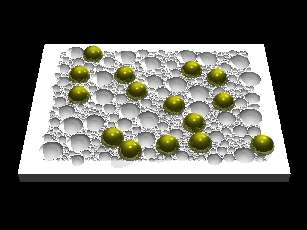
As an example of a complex scene generated by an external program we will next provide a C-program names burbujas.c (bubbles). The program places a number of bubbles at random on a surface of size 1000x750 pixels. Bubbles cannot intersect amongst themselves, so our example code determines random positions and random sizes accordingly. If the new location generated by for a bubble falls near an existing bubble a new position is then computed. The size of the sphere is reduced to make them fit. After a large number of iterations one obtains a surface with almost no free space left. The generation of this particular example requires a lot of computation because as the sequence progresses in becomes harder and harder to fit a new bubble.
Compile and run this program. Redirect the standard output to a file name 'burbujas.inc' where the data for the bubbles remain stored (burbujas > burbujas.inc). The output file contains entries as these:
sphere{<-375, 0,   33> 55.0000000 texture{Gold_Metal}} //(0/1)
sphere{< -86, 0,   62> 55.0000000 texture{Gold_Metal}} //(1/2)
sphere{<-326, 0,  346> 55.0000000 texture{Gold_Metal}} //(2/3)
sphere{< 190, 0, -156> 55.0000000 texture{Gold_Metal}} //(3/4)
sphere{<  62, 0, -293> 55.0000000 texture{Gold_Metal}} //(4/5)
sphere{< 323, 0,  161> 55.0000000 texture{Gold_Metal}} //(5/6)
sphere{< 341, 0,  -15> 55.0000000 texture{Gold_Metal}} //(6/7)
...................
I recommend some patience because it takes a while to generate the output file. At any moment you can interrupt the process and edit the output file to make sure that the last entry line is complete. If not just remove it from the file. The source for pov will the following:
The source code contains again references to the token "clock" but this time its purpose is very different. In this case it does not generate a sequence of images for an animation but four images with very different points of view. The position, angle and aperture of the camera varies among the four images.
In the previous POVRAY article we already mentioned that at some point we would examine examples that explore the possibilities of the camera in POVRAY. Well this is one example. It is quite obvious the differences on the final rendered image according to the specifications of the camera. One can achieve many perspectives according to the angle of aperture: small angle yields far perspectives while wide angles yield close-ups. The maximum angle is 180 degrees, it is a very extreme value because it is hard to distinguish shapes.
The images shown were processed on a Pentium 200 MMX 48MB Ram (398 bogomips). It was executed as suggested by using the tool provided earlier in the series, 'pov':
The parameter passed represent:
The time spend to generate each photogram is considerable. With better quality it would take the following times:
pov burbujas 9 9 1 5 1 5Let us examine now the results. In the first of the four photograms the only variation is the camera setup. (position, angle, orientation, etc)
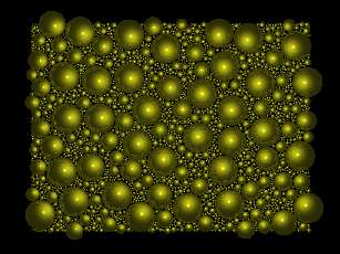
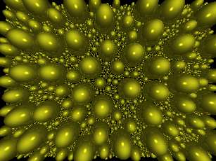
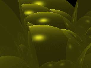
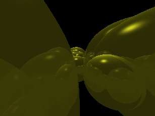
Before showing the last photogram let me go over another issue that is relevant to appreciate this last image, the issue of CPU optimization.
The last photogram is the most complex and POVRAY was not able to optimize it. When confronted by complex compositions the ray-tracer tries to simplify the scene to the simplest common denominator. In previous versions of POVRAY the optimizations had to be done by hand; to this end artists had the directive 'bounded_by' to specify a primitive that would wrap one or more objects. Then the ray-tracer assumed that rays that did not collide with this wrapping would not collide either with any of the objects inside. This is an approximation that saves some processing time. There are very few cases where it is actually useful. As it turns out, our last image is one of those cases!. The last image contains to many objects and is very complex. Therefore it would have been better to manually optimize the composition, for example by grouping bubbles by zones, joining bubbles into compound objects, or even combining all the bubbles in one object but wrapping groups of spheres within the same region using the command 'bounde_by'. The syntax would be:
    union {
    sphere { <x1, y1, z1>, r1 }
    sphere { <x2, y2, z2>, r1 }
    sphere { <x3, y3, z3>, r1 }
    ..........................
    bounded_by { sphere { <xb, yb, zb>, rb } }
  }
The type of manual optimization described can be used with unions and intersections and also with any other object. The user may also select other wrapping primitives, we chose a sphere, however the best results are often obtained with boxes and spheres. If the primitive selected leaves part of the compound object outside the result can be defective.
Once again I would like to stress that the need for manual optimizations is rare. Our last example was conceived with 'bad intentions' beforehand in order to raise the issue. POVRAY automatic optimizer was unable to handle any better the composition. It contains 2154 spheres. The reader could check it out counting them :-).
In our example we have shown how to play with the possibilities of the ray-tracer. Many times the same idea or concept can be implemented in various ways to obtain diverse results and here is where the artist's creativity surfaces.
Povray provides many mathematical functions, some more or less interesting. Unfortunately there is one very interesting function missing. It is the "spline". There is nothing as convenient as tracing with pencil and paper a few points and then applying a function that draws a smooth line across the points. Povray's spline primitive can not be used as a function, instead it generates a line as the basis for building other forms, it would be better if we could apply the spline to any variables we wish. That would allow for example to make the camera follow an arbitrary trajectory. I would also be great if one could implement external functions. To some degree all these can be achieve by using includes and external programming. Under Linux we have a utility named 'spline'. It can be used as a command to generate the desired curve from a set of points. Try to combine this command with external programming, for example to generate animations or camera movement.
I am eager to here from readers and see their compositions, perhaps employing the recursive or loop structures discussed here. Please send me you experiments in compress files. It would be great to collect readers collaborations and organize an exhibition here in the LinuxFocus magazine. I will select the most interesting or imaginative images for the exhibition. Please do not submit images under some kind of commercial for-pay license. If possible send also the sources for the images so that other people can learn from your ideas.
|
Webpages maintained by the LinuxFocus Editor team
© Antonio Castro, FDL LinuxFocus.org |
Translation information:
|
2002-10-22, generated by lfparser version 2.32